Running, Profiling, and Data Analysis on Odo/Frontier
This instructions are for the Odo training system at OLCF. Which is almost identical to Frontier.
Setting up the code
We assume the user has access to the trn047 training account.
-
Access Odo/Frontier
$ ssh USERNAME@odo.olcf.ornl.gov -
Obtain the Gray-Scott.jl code: first access your scratch directory, clone the repository.
cd /gpfs/wolf2/olcf/trn047/scratch/$USER git clone https://github.com/JuliaORNL/GrayScott.jl.git -
Configure the environment: Run the script prepared for this tutorial
GrayScott.jl/scripts/config_odo.shto set up modules, environment, and package dependencies. This is a one-time step and might take a few minutes.source GrayScott.jl/scripts/config_odo.sh#!/bin/bash PROJ_DIR=/gpfs/wolf2/olcf/trn047/scratch/$USER export JULIA_DEPOT_PATH=$PROJ_DIR/.julia GS_DIR=$PROJ_DIR/GrayScott.jl # remove existing generated Manifest.toml rm -f $GS_DIR/Manifest.toml rm -f $GS_DIR/LocalPreferences.toml # good practice to avoid conflicts with existing default modules module purge ROCM_VERSION=7.2.0 # load required modules module load PrgEnv-cray/8.6.0 module load cray-mpich module load rocm/$ROCM_VERSION module load adios2/2.10.0-mpi module load julia/1.13.1 # AMDGPU.jl requires rocm system libraries (default = /opt/rocm) export ROCM_PATH=/opt/rocm-$ROCM_VERSION # Required to point at underlying modules above export JULIA_ADIOS2_PATH=$OLCF_ADIOS2_ROOT # Downloads Julia packages in Project.toml julia --project=$GS_DIR -e 'using Pkg; Pkg.instantiate()' # Set MPIPreferences to use Cray's MPICH in LocalPreferences.toml julia --project=$GS_DIR -e 'using MPIPreferences; MPIPreferences.use_system_binary(mpiexec="srun", vendor="cray")' # Set JACC AMDGPU back end in LocalPreferences.toml. # It will add AMDGPU to Project.toml julia --project=$GS_DIR -e 'using JACC; JACC.set_backend("AMDGPU")' # Verify the packages are installed correctly julia --project=$GS_DIR -e 'using Pkg; Pkg.build()' # Precompile dependencies julia --project=$GS_DIR -e 'using Pkg; Pkg.precompile()'
The JULIA_DEPOT (set by the environment variable JULIA_DEPOT_PATH) is where Julia packages and artifacts (e.g., extra data) will be installed for different local environments. Do not use $HOME for limited performance - not scalable - and storage reasons.
Running jobs
-
Create an area for Gray-Scott runs outside the repository (e.g. run001, future runs will be in run002, run003, etc.)
mkdir run001 -
Copy the Gray-Scott settings file and the job_odo.sh to the run directory
cp GrayScott.jl/examples/settings-file-odo.json run001 cp GrayScott.jl/scripts/job_odo.sh run001 -
Submit your first job to Odo. It should generate an adios bp file output, and total runtime should be around 17 seconds using a single MPI process and AMD GPU.
cd run001 sbatch job_odo.sh -
Check the output files generated by the job with ADIOS2 bpls
bpls -lav gs-1MPI-1GPU-64L-F32-JACC-AMDGPU.bpFile info: of variables: 3 of attributes: 13 statistics: Min / Max double Du attr = 0.2 double Dv attr = 0.1 double F attr = 0.02 string Fides_Data_Model attr = "uniform" string Fides_Dimension_Variable attr = "U" double Fides_Origin attr = {0, 0, 0} double Fides_Spacing attr = {0.1, 0.1, 0.1} string Fides_Variable_Associations attr = {"points", "points"} string Fides_Variable_List attr = {"U", "V"} float U 100*{64, 64, 64} = -0.115931 / 1.46275 float V 100*{64, 64, 64} = 0 / 1.04308 double dt attr = 1 double k attr = 0.048 double noise attr = 0.1 int32_t step 100*scalar = 10 / 1000 string vtk.xml attr = <VTKFile type="ImageData" version="0.1" byte_order="LittleEndian"> <ImageData WholeExtent="0 64 0 64 0 64" Origin="0 0 0" Spacing="1 1 1"> <Piece Extent="0 64 0 64 0 64"> <CellData Scalars="U"> <DataArray Name="U" /> <DataArray Name="V" /> <DataArray Name="TIME"> step </DataArray> </CellData> </Piece> </ImageData> </VTKFile> -
Future runs: repeats steps 1-3 above , and edit the settings file to set the desired parameters for the Gray-Scott simulation.
Lis the number of cells on each direction, Lx = Ly = Lz = L, so L^3 is the total number of cells.plotgapis the number of steps between each visualization output.stepsis the total number of steps to run the simulation.outputis the name of the adios2 output directory dataset (can be visualized with ParaView for small cases)docs.- Other variables might not influence the simulation but can be changed for testing purposes.
{ "L": 64, "Du": 0.2, "Dv": 0.1, "F": 0.02, "k": 0.048, "dt": 1.0, "plotgap": 10, "steps": 1000, "noise": 0.1, "output": "gs-1MPI-1GPU-64L-F32-JACC-AMDGPU.bp", "checkpoint": false, "checkpoint_freq": 700, "checkpoint_output": "ckpt.bp", "restart": false, "restart_input": "ckpt.bp", "adios_config": "adios2.xml", "adios_span": false, "adios_memory_selection": false, "mesh_type": "image", "precision": "Float32" } -
Edit the launch script to request more resources: nodes, gpus, time (follow instructors directions at this point)
 #!/bin/bash
 #SBATCH -A trn047
 #SBATCH -J gs-julia-1MPI-1GPU
 #SBATCH -o %x-%j.out
 #SBATCH -e %x-%j.err
 #SBATCH -t 0:02:00
 #SBATCH -N 1

 date
 #rocminfo

 GS_DIR=/gpfs/wolf2/olcf/trn047/scratch/$USER/GrayScott.jl
 GS_EXE=$GS_DIR/gray-scott.jl

 srun -n 1 --gpus=1 julia --project=$GS_DIR $GS_EXE settings-file-odo.json

 # launch this file with sbatch `$ sbatch job_odo.sh`
Profiling with rocprof
Adding profiling with rocprof allows you to analyze the performance of your Gray-Scott simulation on the GPU. This can help identify bottlenecks and optimize the code for better performance. Since Julia and the GPU backends
-
Adding rocprof to the launch script:
 #!/bin/bash
 #SBATCH -A trn047
 #SBATCH -J gs-julia-1MPI-1GPU
 #SBATCH -o %x-%j.out
 #SBATCH -e %x-%j.err
 #SBATCH -t 0:02:00
 #SBATCH -N 1

 date
 #rocminfo

 GS_DIR=/gpfs/wolf2/olcf/trn047/scratch/$USER/GrayScott.jl
 GS_EXE=$GS_DIR/gray-scott.jl

 srun -n 1 --gpus=1 rocprof -i input.txt -o profiling.csv julia --project=$GS_DIR $GS_EXE settings-file-odo.json

 # launch this file with sbatch `$ sbatch job_odo_rocprof.sh`
where input.txt is the file containing the profiling input counters and profiling.csv is the output file containing the profiling results.
input.txt:
 $ cat input.txt
 # Perf counters group 1
 pmc : Wavefronts VALUInsts SALUInsts SFetchInsts
 # Perf counters group 2
 pmc : TCC_HIT[0], TCC_MISS[0]
profiling.csv:
 Index,KernelName,gpu-id,queue-id,queue-index,pid,tid,grd,wgr,lds,scr,arch_vgpr,accum_vgpr,sgpr,wave_size,sig,obj,Wavefronts,VALUInsts,SALUInsts,SFetchInsts,TCC_HIT[0],TCC_MISS[0]
 0,"gpu_fill_kernel_(CompilerMetadata<DynamicSize, DynamicCheck, void, CartesianIndices<1, Tuple<OneTo<Int64> > >, NDRange<1, DynamicSize, DynamicSize, CartesianIndices<1, Tuple<OneTo<Int64> > >, CartesianIndices<1, Tuple<OneTo<Int64> > > > >, ROCDeviceArray<Float64, 3, 1>, Float64) [clone .kd]",4,0,0,3025283,3025283,17174528,1024,0,0,8,0,16,64,0x0,0x7ffe57ac0880,268352.0000000000,22.9991056523,10.9995528261,4.9998323098,33542,33542
 1,"gpu_fill_kernel_(CompilerMetadata<DynamicSize, DynamicCheck, void, CartesianIndices<1, Tuple<OneTo<Int64> > >, NDRange<1, DynamicSize, DynamicSize, CartesianIndices<1, Tuple<OneTo<Int64> > >, CartesianIndices<1, Tuple<OneTo<Int64> > > > >, ROCDeviceArray<Float64, 3, 1>, Float64) [clone .kd]",4,0,2,3025283,3025283,17174528,1024,0,0,8,0,16,64,0x0,0x7ffe57ac0880,268352.0000000000,22.9991056523,10.9995528261,4.9998323098,33542,33542
The above contains per-kernel profiling results for the specified performance counters. More information available in the AMD rocprof documentation.
Visualizing the output on jupyter-open.olcf.ornl.gov
-
Setup a IJulia kernel for OLCF JupyterHub open and instantiate the project dependencies:
 cd /gpfs/wolf2/olcf/trn047/scratch/$USER/GrayScott.jl/Notebooks/Plot2D.jl
 source config_Odo_IJulia_kernel.sh
#!/bin/bash module load julia/1.13.1 export JULIA_DEPOT_PATH=/gpfs/wolf2/olcf/trn047/scratch/$USER/.julia-notebooks # instantiate project packages: ADIOS2, CairoMakie, IJulia julia --project -e 'using Pkg; Pkg.instantiate()' # configure IJulia kernel for Odo project JUPYTER_KERNEL_FILE=$HOME/.local/share/jupyter/kernels/julia-hpc-sc26-1.13/kernel.json if [ ! -f "$JUPYTER_KERNEL_FILE" ]; then echo "Installing IJulia kernel for julia-hpc-sc26" julia --project -e 'using IJulia; installkernel("julia-hpc-sc26", "--project=@.", env=Dict( "USER" => ENV["USER"], "PATH" => ENV["PATH"], "LD_LIBRARY_PATH" => ENV["LD_LIBRARY_PATH"], "JULIA_DEPOT_PATH" => ENV["JULIA_DEPOT_PATH"], "JULIA_NUM_THREADS" => "8"))' fi # resulting kernel.json cat $JUPYTER_KERNEL_FILE echo "Now log into https://jupyter-open.olcf.ornl.gov/ and select the julia-hpc-sc26 1.13 kernel to run Plot2D.ipynb"The script will output the contents of the resulting
$HOME/.local/share/jupyter/kernels/julia-hpc-sc26-1.13/kernel.jsonfile to verify the kernel installation.The file contents should look similar to the following:
{ "interrupt_mode":"signal", "language":"julia", "argv":["/autofs/nccsopen-svm1_sw/odo/julia-1.13.1/bin/julia","-i","--color=yes","--project=@.","-e","import IJulia; IJulia.run_kernel()","{connection_file}"], "env":{"JULIA_NUM_THREADS":"8","JULIA_DEPOT_PATH":"/gpfs/wolf2/olcf/trn047/scratch/wfg/.julia-notebooks","PATH":"/sw/odo/julia-1.13.1/bin:/opt/conda/bin: ...,"LD_LIBRARY_PATH":"/sw/odo/julia-1.13.1/lib: ..."}, "display_name":"julia-hpc-sc26 1.13" } -
Go to the OLCF JupyterHub Open portal: https://jupyter-open.olcf.ornl.gov/. After signing in and selecting the Onyx Compute resource, select the
julia-hpc-sc26 1.13kernel to run thePlot2D.ipynbnotebook to inspect data fromrun001. -
Browse into the notebook location if it is not immediately visible:
/gpfs/wolf2/olcf/trn047/scratch/$USER/GrayScott.jl/Notebooks/Plot2D.jl/src -
Run the Notebook cells (right triangle or Run menu > Run All Cells) and check you can get to the picture shown below. It might take some time for the packages to be precompiled. The result is a generated set of pdf files containing the 2D
x-yvisualizations of the simulation data on thez=L/2plane This is your first complete workflow from running a Gray-Scott simulation on Perlmutter high-performance computing system and visualizing the results on JupyterHub Open.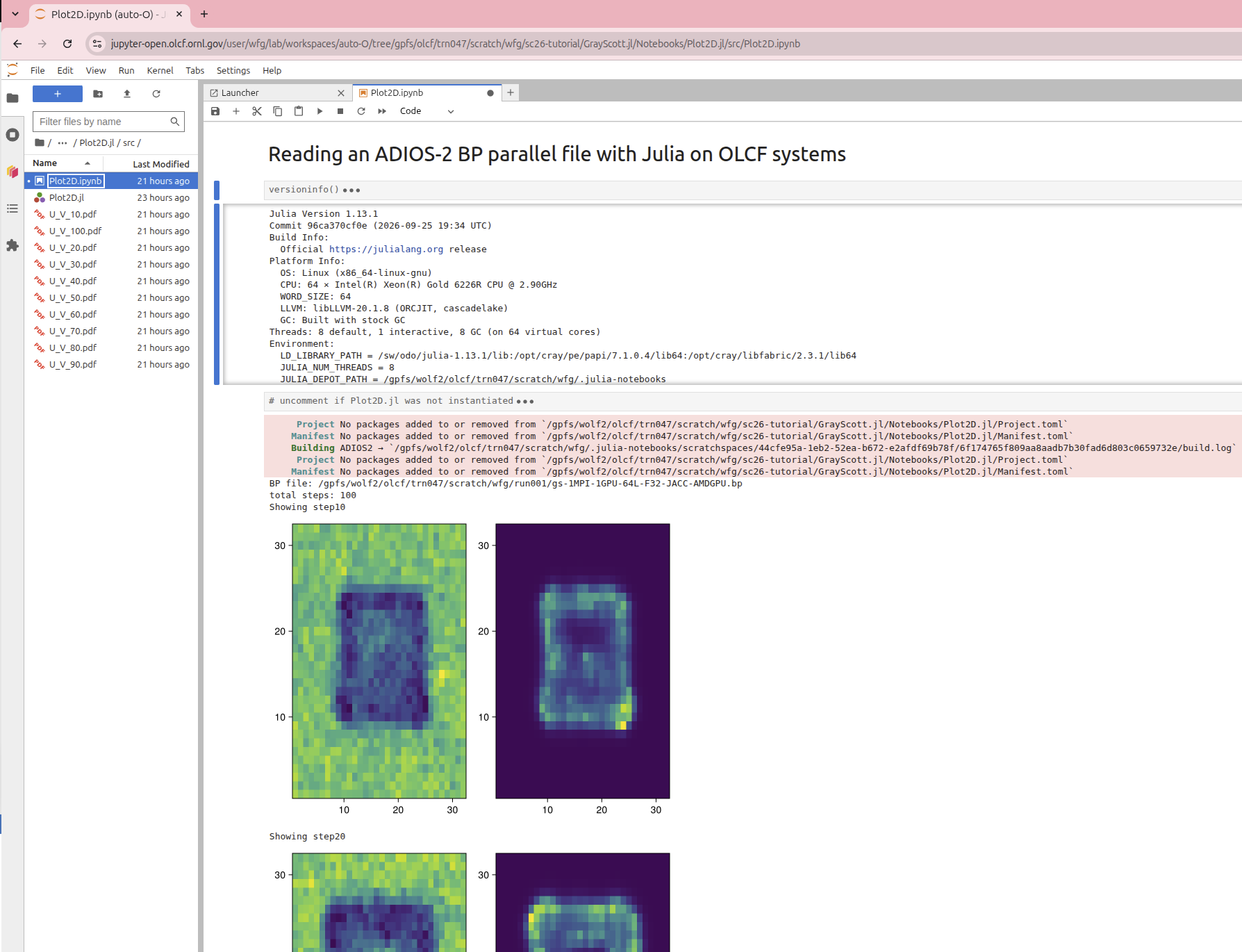 Gray-Scott U and V output visualization using Makie.jl and ADIOS2.jl
-
Congratulations! You have run high-performance computing code and do the data analysis using one language.